In this blog post, I will summarize some ideas on the dynamics of simple excitatory-inhibitory binary network models, their relation to balance and excitability, and what I learnt during the past years. I started working on this topic in 2018, publishing some stuff. I believe that our results highlight some key point of irregular cortical states that are not always taken into account, in particular in more theoretical circles. So if you are into simple models, dynamics, criticality or balance, you might be interested in reading this article.
Also, I believe the story of how I got the results is a fun one and might be motivating for some of you. Let’s get down to it!
Input fluctuations and Jensen’s force
One of the first things I did during my PhD was to try to understand the results of a 2014 Physical Review Letters article by Daniel Larremore and coauthors. It was a simple model of E-I interactions, and the punchline was that inhibition was inducing “ceaseless” activity, which seems to be puzzling. Why did I start with that? To be fair, it was like Pokemon: my PhD supervisor gave me three papers to read and told me to start replicating my favorite one!
The setup is as follows: one has a network of neurons, that can be either active or inactive. Time is discrete. And that a neuron will be active in the next timestep grows as the input to the neuron grows, being capped at one. A neuron with no input (or negative one) has a zero probability of firing. In the original model, the network was random, sparse, directed, and with uniformly distributed coupling weights.
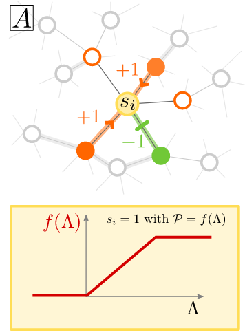
The main plot twist of the PRL paper was the following: the transition to the active phase should happen when the largest eigenvalue of the network becomes larger than 1. Previously, the authors determined a way to obtain analytically this eigenvalue from the network’s average weight coupling. However, when inhibition was introduced, one could find a stable, low amount of activities for apparently subcritical values. The authors were able to identify the source of these activities as input fluctuations…
…but in a very convoluted way. To understand what was going on, I decided to start taking out some ingredients of the network to simplify things. I started removing directionality in the network; then, setting all coupling to be homogeneous, and after that, I fixed the amount of E and I inputs.
In the end, we decided to remove the network completely. Each neuron would choose randomly a fixed number of excitatory and a fixed number of inhibitory cells from the system and compute its input from them. This would happen at every time step. And what changed in the dynamics? Nothing!
The eigenvalue formula used in the PRL paper was returning a kind of “mean-field” approximation, meaning that it was not taking into account input fluctuations. The condition “largest eigenvalue = 1” translates to different critical values of coupling depending on network connectivity. But in simulations, network activity would start always at the same coupling: the one corresponding to a system without inhibition. Therefore, inhibition was not creating ceaseless activity: it was reducing it, but moving the “mean-field” transition towards larger values of the coupling.
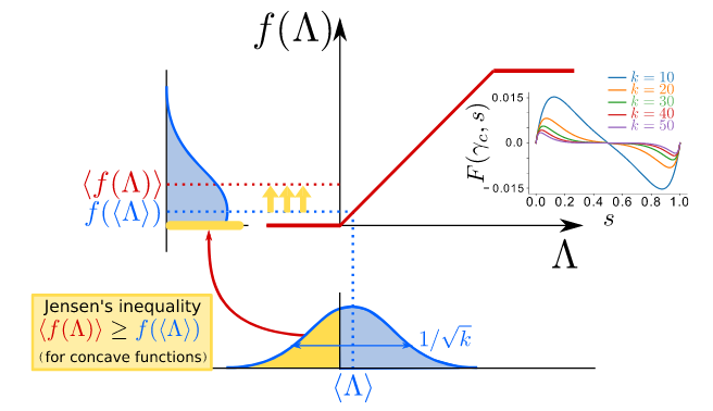
In our simple case where no actual network is used, analytics can be easily done. The probability of taking $n_e$ excitatory neighbours out of a population of size $N_e$ can be written as a binomial distribution. With this, we were able to compute the exact location of the transition as well as the activity phase diagram. We termed this difference between the “mean-field” and the actual result “Jensen’s force” because using Jensen’s inequality one can visualize what happened to the input. Also, we show that all the effects disappear when the network is fully connected, which kills all the input fluctuations.
Years later, I realized that our approach is no different conceptually to that of dynamic mean-field theory. For example, in the works by Brunel and Amit in the early 2000s, what one does is approximate input to neurons with Gaussian white noise, since in a sparse, large network the input is a sum of weakly correlated, random variables. In our case, the simplicity of the dynamics did allow us to use the full distribution of the inputs and obtain exact, closed analytical solutions. However I was not aware of these results when I just started.
Asynchronous irregular state and thermodynamics
One of the interesting things that came out of our study was that activity in the region where “largest eigenvalue < 1” had different dynamical properties than usual active regions. It displayed very low pairwise correlations and it activity was always very low. The low-activity region was sandwiched between two well-defined phase transitions: from no activity to low activity, and then to saturation. That’s what motivated the name “low-activity intermediate” phase in our original 2019 paper.
The fact that the LAI is separated with phase transitions from other usual “active” regions meant that such activity was a thermodynamic phase in its own right, a very interesting fact from a purely physics point of view. This was never reported before us, up to my knowledge. It was similar to a chaotic phase, but there was no need for heterogeneity at all.
![]()
We realized a bit later that in neuroscience such activity is usually called asynchronous state. The fact that we had a model with both usual activity and irregular one was important because we realized the distinction between both was not clear at all in the literature. For example, Benayoun and colleagues in 2010 called “asynchronous irregular” network activity to fluctuations around a low-activity fixed point. But they use a fully connected network, which is completely mean-field: no input fluctuations can be present, and hence the actual irregular activity cannot be present. They had fluctuating low activity, but they had different statistics than Larremore’s one.
One could argue that Benayoun’s model is different to Larremore’s. And to be fair, I always disliked the latter because the units are not quite realistic. The only thing a neurons needs to activativate is to have enough active neighbours, and this is totally independent of neuron’s own state. Hence, a unit can remain active forever, something I never was fond of. On the contrary, Benayoun et al. had a slightly more reasonable model, the stochastic Wilson-Cowan. Since we did show that Jensen’s input fluctuations were responsible for the asynchronous irregular activity, this should be model-independent. I thought it would be cool to replicate my findings in a more realistic model and combine it with avalanches. So there I went.
Excitability shows up
During my PhD I tried for one month to do this and I could never get it. Benayoun had inhibition and balance, so just by making the network sparse it should worked, right? It did not. No matter what I did, there would be always one boring a single absorbing-to-active transition, instead of a nice sandwiched LAI phase.
I forgot about the topic for some time and wrote some philosophical discussion on why or why not should we expect a LAI phase in the stochastic Wilson-Cowan equations in my PhD thesis. Later on, Roberto Corral showed up as a new student in the department at Granada. It is a tradition that we have to be able to simulate a branching process in 1 and 2 dimensions as a warm-up exercise before starting the thesis, so there he went.
Then our supervisor suggested that we could try to use these simulations to create an “E-I branching process”, which at the end of the day turned out to be the stochastic Wilson-Cowan equations. And the question arose again: can we find the LAI phase? My bet was no, since I already tried and failed, but it would be nice if a new person looked at it.
After some failures here and there, Roberto came up with the solution. He told me one day that he found something weird in the dynamics when the coupling among neurons was increased by a lot. Yet, the result was no nice sandwiched LAI phase. What actually happened in the Benayoun et al. model is that most of the system’s dynamics were irregular, and only one transition was present for a large region in the parameter’s space. That’s why I did not see anything: I was looking for two transitions to find a LAI, but I never took the seemingly active phase and wondered: is this irregular? Roberto went further and discovered that the irregular activity was there, in front of us, the whole time. I was biased by the fact that the first time the LAI was between two phases, and never thought it could span such a large region, making it difficult to see it in the graphs.
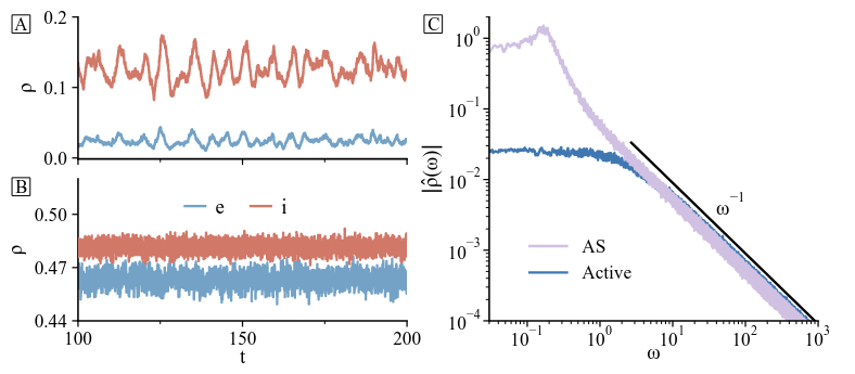
With this new knowledge, I repeated the analytics I did initially for Larremore et al.’s model in the new setup. Roberto performed the simulations, and they matched very well. However, there was something not present before: for some values of the control parameters, we found that the “asynchronous irregular” was not so “asynchronous”, but seemed to have some slow oscillatory ripples. In fact, Fourier transform showed a small peak in frequency, which was not present in our Jensen’s paper. Our results were published some time ago in Phys. Rev. Research.
We were able to relate the oscillations to stochastic amplification of fluctuations, an effect proposed by Jorge Mejías and our supervisor Miguel Ángel to which nobody paid too much attention when it was published more than 10 years ago. Similar mechanisms have been recently independently proposed, including data. The core idea involves the combination of a fixed stable spiral with non-normality.
Think about a Fithugh-Nagumo neuron. One can have a globally stable fixed point, but stability is attained by only one direction in phase space. If the system is perturbed in a perpendicular direction, then it is forced to do a very large excursion (a spike) before coming back to rest. Non-normality measures the time the excursion takes, and how easily a system is perturbed. When combined with a fixed stable spiral, the results are induced oscillations: noise can perturb the system out of equilibrium, which will then slowly come back following the spiral with a given period.
This is exactly what it is happening in the stochastic Wilson-Cowan equations. We were able to use our analytical tools to compute a non-normality measure. The dynamics of the resulting network in a slightly excitable setup look way more accurate (when compared to models such as the classic paper by Renart et al. in 2010 or experimentla data) when compared to previous research.
Also, we were able to replicate results from other recent studies using similar approaches, and explain them all with a “unified” framework in terms of balanced amplification and asynchronous irregular activity. For example, excitability seems to be behind the tilted avalanches in study of de Candia et al., which thoroughly study the stochastic Wilson-Cowan equations. So what’s next?
Reinventing the wheel to improve it
I would like to remark a very recent paper by Menesse and Kinouchi in Phys. Rev. E. They did not know about our previous research and independently arrived at the same results I got by using a model far more complex than the ones I studied. We contacted the authors while the paper was still in preprint stage, and the final version in PRE contains a very complete comparison between our previous research, their model, and other classic papers such as Brunel 2000 which I definitely enjoyed reading. And if you’ve read till here, bet you will like the paper too.
The paper contains some highlights that are not very explicitly discussed in our previous work, such as the interpretation of inhibition as “control parameter” in absorbing-active transitions, and very nice math. The model used by Menesse and Kinouchi includes a refractory period, and a continuous membrane potential, and they were able to push the analytics to get a lot of information. The model itself has been also widely studied by the Brazilian people, including Kinouchi himself and other recent publications by Girardi-Schiappo.
The heterogeneity detour
Now we have understood some nice physical features of the E-I networks, we want to start adding more details. A little example that we checked recently is, what happens if the simple Larremore et al’s network had some spatial connectivity and heterogeneity?
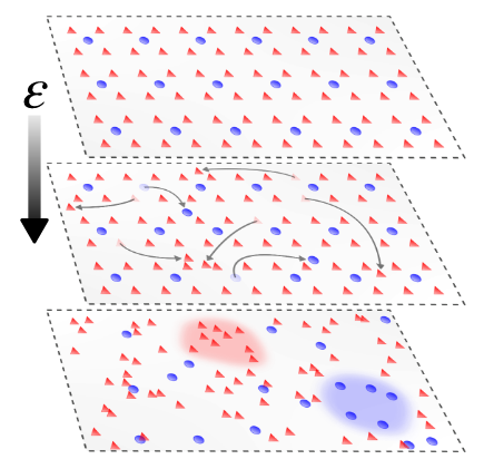
We start with a 2D regular system with balanced weights, but then teleport a fraction of the nodes to random positions in Euclidean space. Connectivity between the nodes is defined using an interaction radius. The initial balance is destroyed when the heterogeneity is added. What happens instead is the emergence of a Griffith’s phase, an entire region with critical-like features.
These happen because, as discussed earlier in this article, Larremore’s dynamics allows for continuous firing of a node if enough neighbours are active. When heterogeneity is included, there’s some chance to have “over-excited” regions with almost-permanent activity, which drive the network for a very long time. However, the balance breaks down. One of our questions was if a plasticity mechanism could bring it back -and in which conditions.
Since the student in charge left the lab, and I had experience with the model already, I helped to finish the study (now a preprint), looking at how inhibitory scaling could do the task. I will skip many of the details, just to remark that plasticity brings the asynchronous state back and I wonder how general this could be, in particular, if the initial network was fully connected.
Small conclusion
I think that the way we attacked this problem is a very nice, simplified way to get corrections to mean-field in networks without having to resort to very technically complicated (i.e. dynamic mean-field, replica…) approaches. Apart from their potential scientific value, I have been always very convinced of the educational power of these derivations: if your compneuro students know how to find fixed points in a dynamical system and what a binomial distribution is, they can analytically find transitions and understand how input fluctuations generate activity (through the Jensen’s force).
Moreover, I learnt a lot of new physics by studying these systems, that might be relevant in other contexts. Many questions remain, like better studying some of the critical transitions between states, the role of excitability or self-organization. But those will be problems for the Victor of the future (and maybe for you too).
See you next time! ~